New post, finally. In this series I’ll be choosing some math and programming problems that I have done that I think were particularly ‘cool’ in that they had elegant solutions, interesting ideas, or neat tricks. They don’t need to be hard to be on this list. This time, the math will be all calculus for the AoPS calculus course I am finishing.
Warmup with Symmetry
Let \(f(x)\) be a continuous function on \([0, a]\), where \(a > 0\), such that \(f(x) + f(a – x) \neq 0\) on \([0, a]\). Evaluate \(\begin{aligned} \int_0^a \frac{f(x)}{f(x) + f(a – x)}dx.\end{aligned}\)
I was stuck on this one for a while, but then I reached the beautiful solution. Reflect the graph across the line \(= \frac{a}{2}\), equivalent to making the substitution \(u = a – x\). The denominator stays unchanged, but the numerator becomes \(f(a – x)\). A reflection does not change area, so geometrically we see the integral is unchanged, and adding them conveniently makes the function
\(\displaystyle \frac{f(x) + f(a – x)}{f(x) + f(a – x)} = 1,\)
so the integral of the sum is $a$ and the answer is \(\boxed{\frac{a}{2}}\).
Putnam 2009 A2
Yes. A Putnam. However difficult, this was a blast. This was done in class but as I missed it that day for a programming competition I decided to crack at it myself.
Functions \(f, g, \) and \(h\) are differentiable on some open interval around $x = 0$ and satisfy the equations and initial conditions
\(\begin{aligned} f’ &= 2f^2gh + \frac{1}{gh}, \ \ \ f(0) = 1, \\ g’ &= fg^2h + \frac{4}{fh}, \ \ \ \ \ g(0) = 1, \\ h’ &= 3fgh^2 + \frac{1}{fg}, \ \ \ \ h(0) = 1.\end{aligned}\)
Find an explicit formula for \(f\), valid in some open interval around \(x = 0\).
Aaargh! We mustn’t fear, there is a fair amount still to go off of. There is noticeable symmetry, so what we can first do is get rid of the denominators to get
\(\begin{aligned} f’gh &= 2f^2g^2h^2 + 1, \\ fg’h &= f^2g^2h^2 + 4, \\ fgh’ &= 3f^2g^2h^2 + 1, \end{aligned}\)
then add them together to get
\(f’gh + fg’h + fgh’ = 6(fgh)^2 + 6.\)
Aha! Notice the left hand side is equal to \((fgh)’\) by the product rule. Though we might be taking a step back from \(f\), it makes sense to define a new function \(y(x) = f(x)g(x)h(x)\). Now, we have the differential equation \(y’ = 6y^2 + 6\) and can solve for $y$. We can separate the variables like so:
\(\displaystyle \int \frac{1}{y^2+ 1} dy = \int 6 dx,\)
and so \(\arctan y = 6x + C, \) and \(y = \tan(6x + C).\) To find \(C\), recall from the initial conditions that \(y(0) = 1,\) so \(\displaystyle C = \frac{\pi}{4}.\)
Now we need \(f\). To find it, we take the first equation with \(f\) and \(f’\) and put \(y\) in it. The rewritten equation becomes
\(f’ = 2fa + \frac{f}{a}.\)
We’re close! To solve this differential equation, we divide both sides by \(f\) so the LHS becomes \(\displaystyle \frac{f'(x)}{f(x)}\) and integrates to simply \(\log |f(x)|.\) The RHS is
\(2a + \frac{1}{a} = 2\tan(6x + \frac{\pi}{4}) + \cot(6x + \frac{\pi}{4}),\)
So integrating both sides gives
\(\log |f(x)| = -\frac{1}{3}\log \cos(6x + \frac{\pi}{4}) + \frac{1}{6}\log \sin(6x + \frac{\pi}{4}) + C.\)
Combining logs and exponents, we find that
\(\log |f(x)| = \log \left(\frac{\sin(6x + \pi/4)}{\cos^2(6x + \pi/4)}\right)^\frac{1}{6} + C.\)
So,
\(f(x) = e^C\left(\frac{\sin(6x + \pi/4)}{\cos^2(6x + \pi/4)}\right)^\frac{1}{6}.\)
Putting in \(f(0) = 1\), we find that $\latex \displaystyle e^C = 2^{-\frac{1}{12}}$, so our final answer is
\(\boxed{f(x) = 2^{-\frac{1}{12}}\left(\frac{\sin(6x + \pi/4)}{\cos^2(6x + \pi/4)}\right)^\frac{1}{6}}.\)
‘Simple’ Integral
Evaluate
\(\displaystyle \int_0^1 \log x\log(1 – x) dx.\)
Me see product, me integrate by parts! Unfortunately, that ship has sailed: we don’t know how to integrate a logarithm. Whatever should we do?
This one’s for the swifties: we can try using a Taylor Series. The situation may look bleak, but we can at least integrate polynomials.
The Taylor Series of \(\log(1 + x)\) around \(x = 0\) is
\(\displaystyle x\ – \frac{x^2}{2} + \frac{x^3}{3}\ – \frac{x^4}{4} + \cdots\)
So substituting $-x$ instead gets the Taylor Series of \(\log(1 – x)\) around \(x = 0\) to be
\(\displaystyle -x\ – \frac{x^2}{2}\ – \frac{x^3}{3}\ – \frac{x^4}{4}\ – \cdots = -\sum_{n = 1}^\infty \frac{1}{n}x^n.\)
We can put this into the integral and pull the infinite sum out in front (note that the integral of a limit of functions is not equal to the limit of the integrals, but it is ok in this case). NOW we can use integration by parts. In \(\displaystyle \int_0^1 x^n\log x dx,\) we set \(u = \log x\) and \(dv = x^ndx\). Then, we get
\(\displaystyle \int_0^1 x^n\log x dx = \left.\frac{1}{n + 1}x^{n + 1}\log x \right|_0^1 – \frac{1}{n + 1}\int_0^1 x^ndx.\)
The first term is undefined as the lower limit makes the antiderivative go to \(0\cdot (-\infty)\), so we have to rewrite this as a limit:
\(\displaystyle \left.\frac{1}{n + 1}x^{n + 1}\log x \right|_0^1 = 0\ – \frac{1}{n + 1}\lim_{x \to 0^+}x^{n + 1}\log x.\)
We love using L’Hôpital’s Rule to deal with indeterminate forms, so to use it we rewrite \(x^{n + 1}\) as \(\displaystyle \frac{1}{x^{-n – 1}}.\) This gives us
\(\displaystyle \frac{1}{n + 1}\lim_{x \to 0^+}x^{n + 1}\log x = \frac{1}{n + 1}\lim_{x \to 0^+} \frac{\frac{1}{x}}{(-n\ – 1)x^{-n – 2}} = \frac{1}{(n + 1)^2}\lim_{x \to 0^+}x^{n + 1} = 0.\)
So, that gets rid of the first term. The second term is much easier: It’s just a case of the power rule, getting us \(\displaystyle \int_0^1 x^n\log x dx = -\frac{1}{(n + 1)^2}.\) Therefore, the original integral is just equal to
\(\displaystyle \sum_{n = 1}^\infty \frac{1}{n(n + 1)^2}.\)
The obvious step is to now take partial fractions. The sum becomes
\(\displaystyle \sum_{n = 1}^\infty \left(\frac{1}{n}\ – \frac{1}{n + 1}\right) – \sum_{n = 1}^\infty \frac{1}{(n + 1)^2}\)
The first sum telescopes to \(1\), and the second is a well-known result from the Basel Problem. So, our final answer is
\(\displaystyle \int_0^1 \log x\log(1 – x) dx = \boxed{2\ – \frac{\pi^2}{6}}.\)
ABC366 F – Maximum Composition
You are given \(N\) linear functions \(f_1, f_2,\dots, f_N,\) where \(f_i(x) = A_i(x) + B_i.\) Find the maximum possible value of \(f_{p_1}(f_{p_2}(\dots f_{p_K}(1)\dots))\) for a sequence \(p = (p_1, p_2, \dots, p_K)\) of \(K\) distinct integers from \(1\) to \(N\).
Constraints
- \(1 \leq N \leq 2\times 10^5\)
- \(1 \leq K \leq \text{min}(N, 10)\)
- \(1 \leq A_i, B_i \leq 50 (1\leq i \leq N)\)
- All input values are integers.
- Time limit: 2 seconds
As \(N\) is really large, this leads us to think about some dynamic programming solution. However, the order in which we use the functions matters, so we have to think about how we can sort the functions so that they always produce the largest value. To do this, consider 2 functions \(f_i(x)\) and \(f_j(x).\) Assume \(f_i(f_j(x)) > f_j(f_i(x)).\) Then,
\(\begin{aligned}A_iA_jx + A_iB_j + B_i &> A_jA_ix + A_jB_i + B_j, \\ A_iB_j – B-j &> A_jB_i – B_i, \\ B_j(A_i – 1) &> B_i(A_j – 1).\end{aligned}\)
This can be our sorting function, which ensures the last functions we use will have a bigger impact. Now, after the sort, it’s a simple matter to iterate through each function and for each one iterate through the number of functions used so far. If dp[i][j] is the maximum answer after using \(j\) functions from the first \(i,\) then the transition is
dp[i][j + 1] = max(dp[i][j + 1], dp[i - 1][j] * a[i] + b[I].
Here in my code I’ve simply used two vectors and swapped them around because you do have to copy over their contents after each iteration so this saves some code and also space.
#include <bits/stdc++.h>
#define int long long
using namespace std;
int n, k;
struct func {
    int a, b;
} f[200001];
bool cmp (func p, func q) {
    return (p.a - 1) * q.b < (q.a - 1) * p.b;
};
signed main() {
    cin >> n >> k;
    for (int i = 1; i <= n; i++) cin >> f[i].a >> f[i].b;
    sort(f + 1, f + n + 1, cmp);
    vector<int> dp(k + 1, -1e9);
    dp[0] = 1;
    for (int i = 1; i <= n; i++) {
        vector<int> nxt = dp;
        for (int j = 0; j < k; j++) {
            if (dp[j] == -1e9) continue;
            nxt[j + 1] = max(nxt[j + 1], dp[j] * f[i].a + f[i].b);
        }
        dp = nxt;
    }
    cout << dp[k];
    return 0;
}
ABC358 G – AtCoder Tour
You have an \(H\times W\) grid with an integer $A_{i, j}$ written in the cell on the \(i\)-th row and \(j-\)th column. Takahashi starts at $(S_i, S_j)$ and repeats the following action \(K\) times:
Either stay in the current cell, or move to an edge-adjacent cell. In both cases, gain the value of the cell he is in after the action.
Find the maximum value he can gain.
Constraints
- \(1 \leq H, W \leq 50\)
- \(1 \leq K \leq 10^9\)
- \(1 \leq A_{i,j} \leq 10^9\)
- Time limit: 2 seconds
Notice how there can be only a maximum of \(2500\) cells yet \(K\) can be up to 1 billion. There seems little use then to move Takahashi more than \(HW\) times, because he can just sit at the cell with the highest value and profit from there instead of repeatedly visiting the same cells. So, let’s find the maximum value one can get from reaching each cell \((i, j)\) after \(t\) actions as dp[t][i][j], then if we stay there the value gained will be dp[t][i][j] + (k - t) * a[i][j]. The code is simple:
#include <bits/stdc++.h>
#define int long long
using namespace std;
int h, w, k, sx, sy, a[51][51], ans, f[2510][51][51];
int dx[] = {0, 1, 0, -1}, dy[] = {1, 0, -1, 0};
signed main() {
    cin >> h >> w >> k >> sx >> sy;
    for (int i = 1; i <= h; i++)
        for (int j = 1; j <= w; j++)
            cin >> a[i][j];
    memset(f, -0x3f, sizeof(f));
    f[0][sx][sy] = 0;
    for (int t = 0; t <= min(k, h * w); t++)
        for (int i = 1; i <= h; i++)
            for (int j = 1; j <= w; j++) {
                ans = max(ans, f[t][i][j] + (k - t) * a[i][j]);
                for (int d = 0; d < 4; d++) {
                    int nx = i + dx[d], ny = j + dy[d];
                    if (nx < 1 || nx > h || ny < 1 || ny > w) continue;
                    f[t + 1][nx][ny] = max(f[t + 1][nx][ny], f[t][i][j] + a[nx][ny]);
                }
            }
    cout << ans;
    return 0;
}
ABC232 G – Modulo Shortest Path
This one was tough! I encountered it in a mock competition and only managed to solve 4 of the 10 test cases that had small numbers, but that was my teacher’s intention anyway. There was no way I could of thought of this myself, but now I have some more experience with this kind of approach!
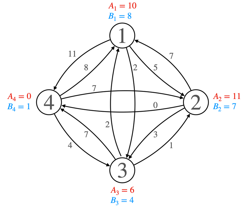
There is a directed graph with \(N\) vertices labeled \(1, 2,\dots, N\). Vertex \(i\) has 2 numbers \(A_i\) and \(B_i\) associated with it, and the directed edge from \(i\) to \(j\) is \((A_i + B_j) \mod M,\) where \(M\) is given. Find the shortest path from \(1\) to \(N\).
Constraints
- \(2\leq N \leq 2\times 10^5\)
- \(2\leq M \leq 10^9\)
- \(0\leq A_i, B_j < M\)
- Time limit: 3 seconds
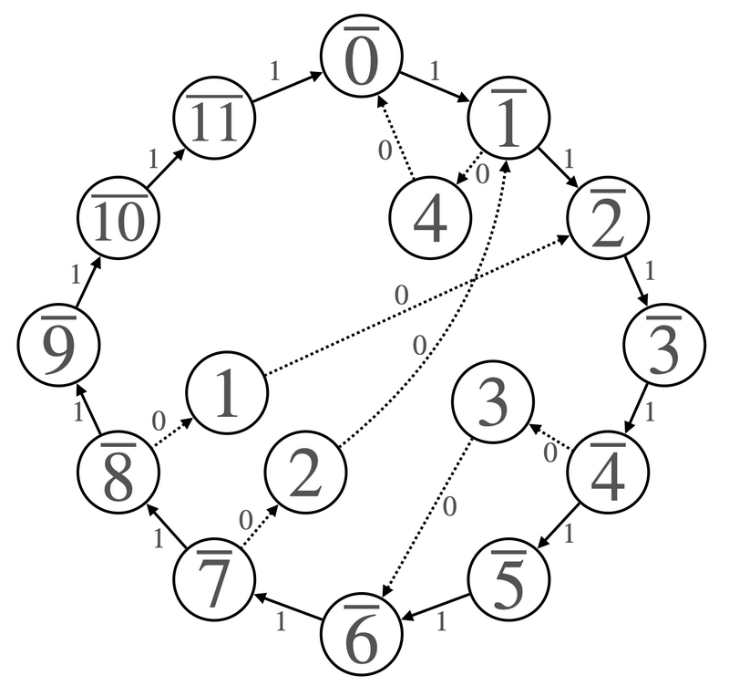
Dijkstra’s algorithm works for shortest paths but will take \(\Theta(N^2\log N)\) which will not be fast enough. We will have to modify the graph somehow to have \(O(N)\) vertices and edges. To do this, we create the following graph \(G’\), exploiting the cyclical nature of the modulo operation:
- In addition to the original \(N\) vertices, create \(M\) new ones labeled \(0′, 1′, 2′,\dots, (M\ – 1)’\).
- Create a directed edge of weight 1 from \(i’ \) to \((i + 1)’\) for \(0 \leq i < M – 1\) and also from \((M – 1)’\) to \(0’\).
- Create a directed edge from \(i\) to \(((-A_i)\mod M)’\) of weight 0 for \(1 \leq i\leq N\).
- Create a directed edge from \(B_i\) to \(i\) of weight 0 for \(1 \leq i\leq N\).
Believe it or not, this is all we need to eliminate the modulo operation! Test for yourself and see what happens. From the official editorial, here is a diagram to show this.

becomes

Here is a more formal proof. When \(A_i =0\), there is no change to the edge length. Otherwise, we will end up on the outer ‘ring’ at \((M – A_i)’\). Now, we have 3 cases:
Case 1: \(B_j = M – A_i\), so the distance on \(G’\) will be zero. Also, \(B_j + A_i = M,\) so the edge on \(G\) will also have length 0, so they are the same.
Case 2: \(B_j > M – A_i\), so the distance on \(G’\) will be \(B_j – M + A_i.\) Also, \(B_j + A_i > M\), so the edge on \(G\) will have length \(A_i + B_j – M,\) which is the same.
Case 3: \(B_j < M – A_i\), so the distance on \(G’\) will be \(M – (M – A_i) + B_j = A_i + B_j.\) Also, \(B_j + A_i < M\), so the edge on \(G\) will have length \(A_i + B_j,\) which is the same.
Now, there is still one problem, which is that \(M\) can be massive, so there will still be too many vertices for Djikstra. However, \(N\) won’t be that large, and so we can just get run through the outer ring, getting rid of the unused vertices and then making the remaining edges longer. Also, we can get rid of the inner nodes entirely. Here is the code:
#include <bits/stdc++.h>
#define int long long
#define pii pair<int, int>
using namespace std;
int n, m, a[200001], b[200001], cnt, s, e, dist[400001];
map<int, int> mp;
vector<int> nums;
vector<pii> graph[400001];
bool vis[400001];
priority_queue<pii, vector<pii>, greater<pii>> pq;
signed main() {
    cin >> n >> m;
    for (int i = 1; i <= n; i++) {
        cin >> a[i];
        a[i] = (m - a[i]) % m;
        if (!mp[a[i]]) {
            mp[a[i]] = ++cnt;
            nums.push_back(a[i]);
        }
    }
    for (int i = 1; i <= n; i++) {
        cin >> b[i];
        if (!mp[b[i]]) {
            mp[b[i]] = ++cnt;
            nums.push_back(b[i]);
        }
        graph[mp[b[i]]].push_back(make_pair(mp[a[i]], 0));
    }

    s = mp[a[1]], e = mp[b[n]];
    sort(nums.begin(), nums.end());
    for (int i = 0; i < cnt - 1; i++) {
        int cur = nums[i], nxt = nums[i + 1];
        graph[mp[cur]].push_back(make_pair(mp[nxt], nxt - cur));
    }
    graph[mp[nums[cnt - 1]]].push_back(make_pair(mp[nums[0]], (nums[0] + m - nums[cnt - 1]) % m));

    for (int i = 1; i <= cnt; i++) dist[i] = 1e18;
    dist[s] = 0;
    pq.push(make_pair(0, s));

    while (!pq.empty()) {
        int v = pq.top().second;
        pq.pop();
        if (vis[v]) continue;
        vis[v] = true;
        for (pii j : graph[v]) {
            int to = j.first, w = j.second;
            if (dist[v] + w < dist[to]) {
                dist[to] = dist[v] + w;
                pq.push(make_pair(dist[to], to));
            }
        }
    }
    cout << dist[e];
    return 0;
}

